Research Highlight 1: DNS and measurements of scalar transfer across an air-water interface during inception and growth of Langmuir circulation
Introduction: As part of National Science Foundation Award #1235039 , we have successfully run multiple direct numerical simulations (DNS) of turbulent flow generated by the interaction between a wind-driven shear current and centimeter-scale surface gravity-capillary waves often occurring in lakes and oceans (Figure 0). The simulations have been performed with a finite volume multi-fluid (air-water) incompressible Navier-Stokes solver resolving the wind and wave-driven air-water coupled molecular boundary layers and the interface between the air and water.
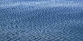
Figure 0: Gravity-capillary waves in the ocean. The water side-turbulence generated by these waves controls the tranfer rate of gases such as CO2 from the air-side to the water-side. The turbulence is characterized by turbulent diffusion serving as the mechanism of gas transfer from the air-side to the water-side. Increased levels of CO2 in the ocean makes the water more acidic significantly impacting the biology in the ocean.
For slightly soluble gases in water such as CO2, the water side turbulence controls the gas transfer rate from the air to the water side. We have focused on comparing scalar (gas) flux across the air-water interface and vertical transport of the scalar throughout the water side calculated in the DNS of the deforming air-water interface (deforming interface case) previously described with those calculated from a similar DNS but in which the interface is intentionally held flat. The goal of this comparison is to understand the effect of Langmuir turbulence in the deforming interface case on scalar flux across the air-water interface and on vertical transport relative to the effect of pure shear turbulence generated by the wind when the interface is held flat. Langmuir turbulence in the water side is generated via the interaction between the Stokes drift current induced by the gravity-capillary waves (characterizing the air-water interface) and the wind-driven current.

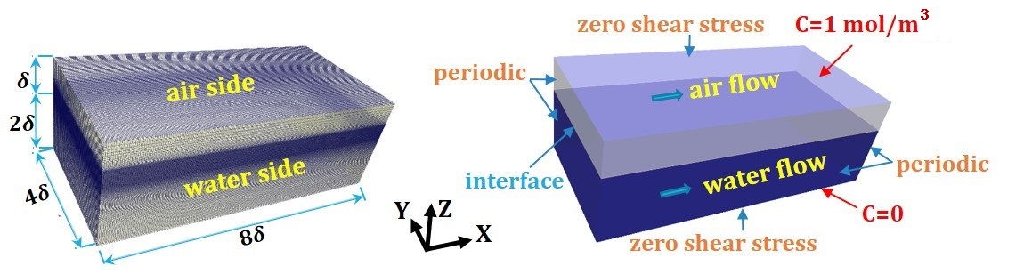
The computational mesh shown in Figure 1a consisted of 200 by 100 by 60 grid points on the air side and 200 by 100 by 120 grid points on the water side in the streamwise, spanwise and vertical directions respectively (3.6 million grid points in total). The computational mesh is uniform along the streamwise and spanwise directions, while a gradual mesh refining scheme was applied in which the vertical mesh size becomes smaller in the approach to the air-water interface from either the water side or the air side (see Figure 1a). This meshing scheme was purposely used to resolve the air-water interface including centimeter-scale interfacial deformations as well as the molecular sub-layers in the air- and water-sides. The grid resolution for this mesh is between approximately 0.006 centimeters (near the air-water interface) and 0.05 centimeters (near the top and bottom of the domain).
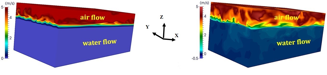
Figure 2. a) Instantaneous snapshot of streamwise (x) velocity field distribution within the domain showing the turbulence in action within the air side and the water at rest as initial conditions. b) Instantaneous snapshot of streamwise velocity field distribution within the domain showing turbulence in action within both the air and water sides after 5s.
The initial condition for scalar (gas) concentration was C = 1 mol/m3 in the air side and C = 0 in the water side for all cases. At the top of the domain (at the top of the air side) C was set to 1 mol/m3 and at the bottom of the domain (the bottom of the water side) C was set to 0, ensuring a flux of scalar from the air side to the water side (Figure 1b).
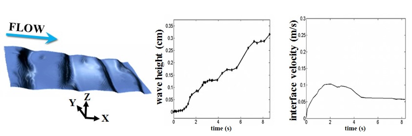
Figure 3. Left panel: the instantaneous air-water interface in DNS at t=2.5s. Middle panel: time series of the simulated maximum air-water interfacial wave heights. Right panel: time series of the simulated average streamwise velocity on the air-water interface.
A second simulation was made similar to the one previously described but in which the air-water interface was held intentionally flat. Instantaneous snapshots of downwind (streamwise) vorticity from this flat interface case are shown on Figures 4a and 4b and the corresponding results from the deforming interface case (with corresponding interface deformation or wave field shown in Fig. 3) are shown on Figures 4c and 4d. The deforming interface case is characterized by Langmuir turbulence consisting of Langmuir cells aligned in the direction of the wind and growing in the cross-stream direction and in depth whereas the simulation with the flat interface shows smaller and less intense near-surface vortices.
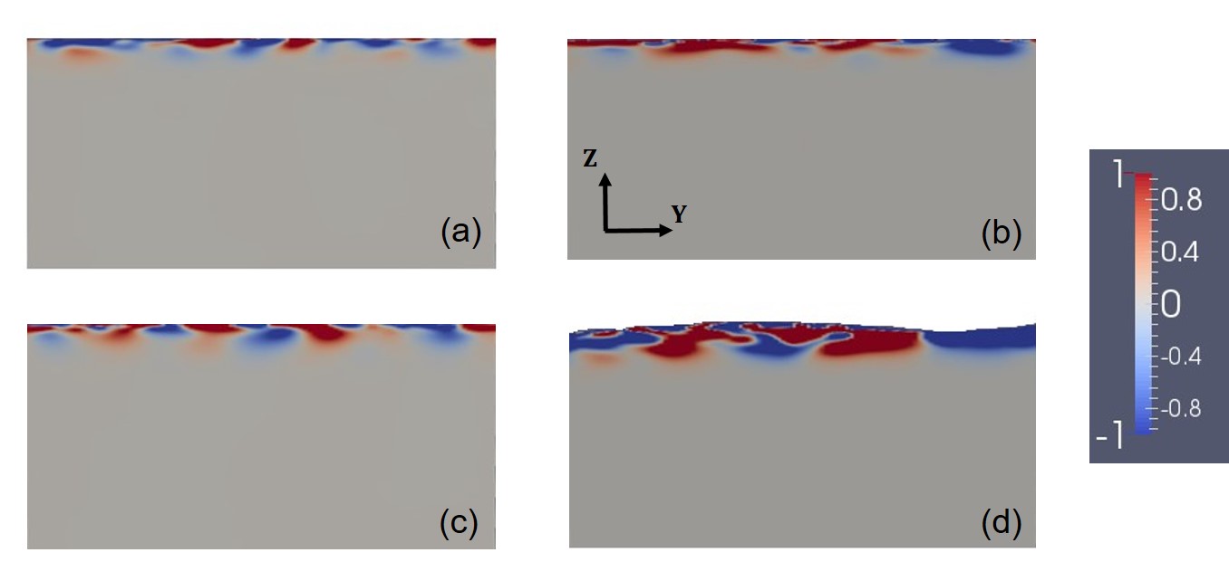
Figure 4: Instantaneous streamwise vorticity (s-1) from DNS with air-water interface held flat at a) t = 1s and b) t = 3s. Instantaneous streamwise vorticity (s-1) from DNS with freely deforming air-water interface at c) t = 1s and d) t = 3s. The latter ((c) and (d)) show evolution of Langmuir turbulence while the former ((a) and (b)) show evolution of shear turbulence.
Prior to the transition to Langmuir turbulence which was determined to be at approximately t=2.5 s, both cases simulated (flat and deforming interface simulations) were compared in terms of depth profiles of mean scalar concentration in the water column. It was found that both cases possess similar concentration profiles through t = 2.5 seconds (not shown). However, for times greater than 2.5 seconds, the Langmuir turbulence and associated Langmuir cells in the deforming interface case generate greater vertical transport than the shear-generated turbulence in the flat interface case. From the depth profiles and instantaneous contours of scalar concentration shown in Figure 5, we can conclude that the Langmuir turbulence penetrates deeper than the shear turbulence thus the Langmuir turbulence is able to transport higher concentration fluid to greater depths. Note that as time progresses the difference between Langmuir turbulence penetration in the deforming interface case and the shear turbulence penetration in the flat interface case becomes more significant.
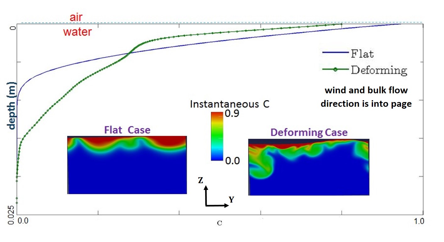
Figure 5: Depth profiles (averaged over streamwise and spanwise directions) and instantaneous snapshots of scalar concentration at time t = 4s in the simulation with a deforming interface and the simulation with a flat interface.
Time series of the spatially (streamwise/cross-stream) averaged scalar flux across the wind-driven air-water interface for the flat and deforming interface cases are shown in Figure 6. A dramatic explosion or spike of scalar flux is observed in the deforming interface case at approximately t=2.5s when the flow transitions to Langmuir turbulence. In contrast, such a sudden increase in scalar flux is noticeably absent in the flat interface case. After this spike, the average scalar flux obtained in the deforming interface case decreases significantly but stabilizes at a mean value approximately two times greater than the scalar flux obtained in the flat case. In the field (i.e. in lakes and oceans), it is likely that such gas flux spikes are correlated with wind transients or gusts and thus might be a dominant contributor to the long-term time-averaged gas flux.
Lastly, we calculate transfer velocity a measure of scalar transfer efficiency:
where is the unit normal to the interface,
is the gradient of the scalar concentration at the interface on the water side,
is concentration on the interface,
is bulk concentration calculated as
with denoting the average over streamwise and cross-stream directions, and
is streamwise velocity. The transfer velocity is a quantity of interest as parameterizations of the gas flux across the air-water interface in climate models and ocean circulation models are often expressed in terms of the transfer velocity with the latter parameterized in terms of wind and wave field characteristics. Due to the enhanced vertical transport induced by the Langmuir turbulence and associated cells, the bulk concentration is significantly greater in the interface deforming case compared to the flat interface case (Figure 7). Ultimately this leads to a greater transfer velocity (
) in the deforming interface case (Figure 8), as
is inversely proportional to the difference between concentration at the interface and bulk concentration (see equation for
above).
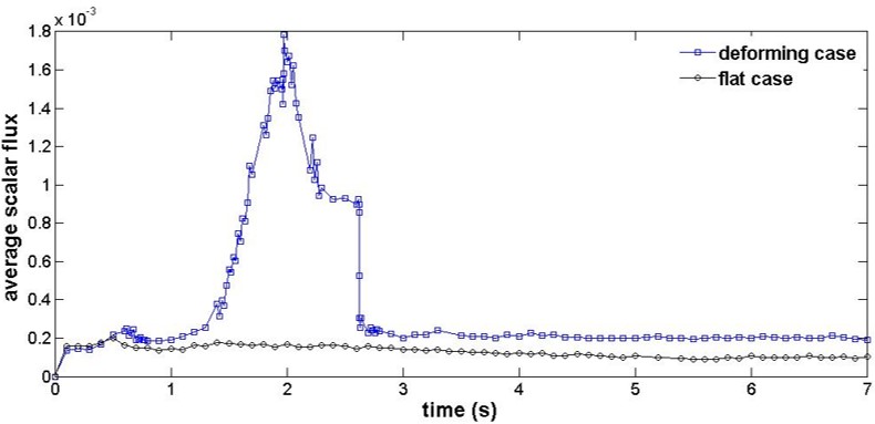
Figure 6: Scalar flux through the air-water interface: where
is the unit normal to the interface and
is the gradient of the scalar concentration at the interface on the water side. The flux is averaged over the interface.
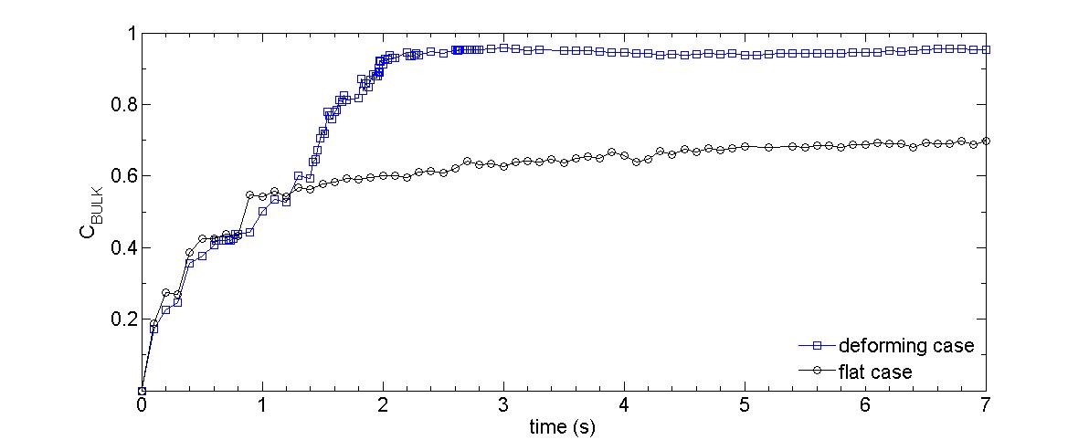
Figure 7: Bulk concentration of the air-water interface
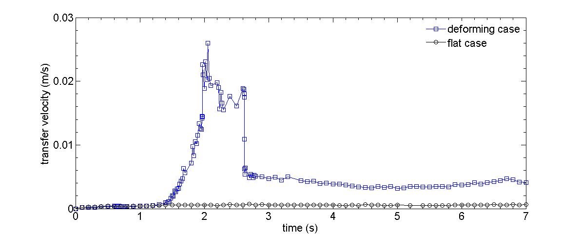
Figure 8: Transfer velocity averaged over the interface
Summary: The deforming interface and associated Langmuir turbulence play important roles in determining scalar flux across the interface and subsequent vertical transport of the scalar. Transition to Langmuir turbulence was observed to be accompanied by a spike in gas flux characterized by an order of magnitude increase. These episodic flux increases, if linked to gusts and unsteadiness in the wind field, are expected to be an important contributor in determining the long-term average of the air-sea fluxes. Finally, vertical transport induced by the Langmuir cells was seen to enhance bulk concentration throughout the water column which ultimately enhances transfer velocity.